=======================================================================
Cybernetics in the 3rd Millennium (C3M) Volume 14 Number 1, Dec. 2017
Alan B. Scrivener — www.well.com/user/abs — mailto:abs@well.com
========================================================================
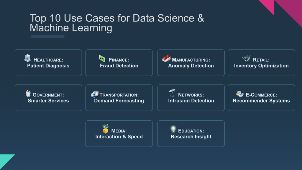 illustration from dzone.com
( dzone.com/articles/top-10-machine-learning-use-cases-part-1 )
In this issue:
illustration from dzone.com
( dzone.com/articles/top-10-machine-learning-use-cases-part-1 )
In this issue:
Short Subjects
 "Fractured Flickers" letterhead with Theda Bara
(artofjayward.blogspot.com/2015/06/fractured-flickers.html)
"Fractured Flickers" letterhead with Theda Bara
(artofjayward.blogspot.com/2015/06/fractured-flickers.html)
- book review: Superforecasting (2016) by Philip E. Tetlock and Dan Gardner
( www.amazon.com/exec/obidos/ASIN/0804136718/hip-20 )
This book is about keeping forecasters honest, quantified and verifiable, and keeping
track of all of their forecasts to avoid what I call "the error of the missing denominator."
It's also about improving forecast quality.
Author Tetlock helped found the Good Judgment Project to promote these goals.
( en.wikipedia.org/wiki/The_Good_Judgment_Project )
It also makes the important distinction between foxes and hedgehogs, expanding on ideas
in a 1953 book by Isaiah Berlin
( en.wikipedia.org/wiki/The_Hedgehog_and_the_Fox )
based on a fragment of the Greek poet Archilochus which says: "The fox knows many things,
but the hedgehog knows one big thing." It is claimed that superforecasters are foxes.
- book review: The Phoenix Project: A Novel about IT, DevOps, and Helping Your
Business Win (2104) by Gene Kim, Kevin Behr and George Spafford
( www.amazon.com/exec/obidos/ASIN/0988262509/hip-20 )
I'm always tickled when a novel comes along which fairly painlessly teaches something.
In this case it's about my own career backyard: Information Technology (IT). A lot of
ugly truths are trotted out in this book that I haven't seen anywhere else in print.
- Web3D is here at last: X3DOM
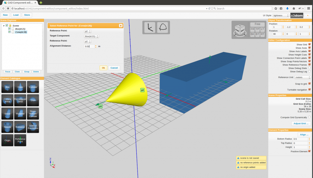 For decades a project called Web3D has popped up at the SIGGRAPH conference and elsewhere,
offering the goal of interactive 3D graphics in a browser with no plug-ins needed. Every
time I checked in they were "almost there." Well, finally, a solution exists, provided
you use a recent version of Chrome or other post-modern browsers. One JavaScript
implementation is X3Dom. See if the example below works for you.
( examples.x3dom.org/example/RadarVolumeStyle/ )
I've been playing with this tech and will report soon. It's been a goal of mine since
forever to write web articles about Bucky Fuller's geometries and have in-line
interactive 3D illustrations.
Meanwhile there's a lot of info available.
( www.x3dom.org/examples/ )
For decades a project called Web3D has popped up at the SIGGRAPH conference and elsewhere,
offering the goal of interactive 3D graphics in a browser with no plug-ins needed. Every
time I checked in they were "almost there." Well, finally, a solution exists, provided
you use a recent version of Chrome or other post-modern browsers. One JavaScript
implementation is X3Dom. See if the example below works for you.
( examples.x3dom.org/example/RadarVolumeStyle/ )
I've been playing with this tech and will report soon. It's been a goal of mine since
forever to write web articles about Bucky Fuller's geometries and have in-line
interactive 3D illustrations.
Meanwhile there's a lot of info available.
( www.x3dom.org/examples/ )
- a short story: The Boomertown Rats
A dear friend of mine, Phil Cohen, passed away about two years ago, and about one year ago
I finished a science fiction short story written in his honor. It's got some cybernetics
in it: darknets, ad hoc currencies, network effects...
( people.well.com/user/abs/Writing__/Fiction/ShortStories/BR/br.html )
- Orlando Attractions on a Deck of Cards
a research project by Alan B. Scrivener
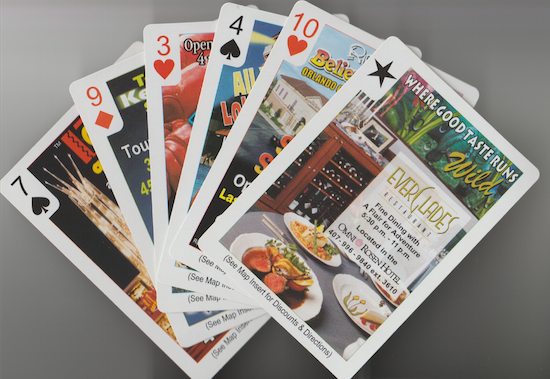 This silly little project doesn't have much to do with cybernetics (except, of course,
that everything does) but it has some interesting raw data, and I found it amusing to do.
Sometimes research is therapeutic for me, and I did this project mostly over the 4th of
July weekend 2017, entirely for fun.
Quote:
This silly little project doesn't have much to do with cybernetics (except, of course,
that everything does) but it has some interesting raw data, and I found it amusing to do.
Sometimes research is therapeutic for me, and I did this project mostly over the 4th of
July weekend 2017, entirely for fun.
Quote:
"About 2000 or early 2001 I visited Orlando for a combined family vacation and business
trip, and ended up picking up a deck of Orlando area promotional cards. It was a real
deck of cards, but had a local attraction or tourist-oriented business on each one.
There was also a map, and the cards keyed into the map. I thought it was a clever gimmick,
and I saved the box with the cards and map inside.
Now, about 17 years later, I became curious which businesses had survived, and so I did
some web research and compiled the following table..."
( people.well.com/user/abs/Writing__/Nonfiction/Orlando/cards.html )
- SoCal Aerospace History Project
In the last few months I've been working on a research project into the history of Southern
California's aircraft and space industries. Again, there isn't a direct connection to
cybernetics (besides the development of self-aiming anti-aircraft guns), but there's
a lot of raw data. The final product will be a series of video blogs, but I'm sharing the
work-in-progress research.
( people.well.com/user/abs/Writing__/Nonfiction/Vlogs/SoCal_aviation.html )
- Dr. Lawrence J. Fogel
 Dr. Lawrence J. Fogel portrait at asc-cybernetics.org
( www.asc-cybernetics.org/foundations/Fogel.htm )
Demonstrating once agin that everything is connected, I found one particular overlap
between cybernetics and SoCal aerospace history. Dr. Lawrence J. Fogel was a Design
Specialist for Convair, a pioneering SoCal aircraft company. He was an early practitioner
of Human Factors Engineering and Artificial Intelligence (AI). He authored the book
"Artificial Intelligence Through Simulated Evolution" (1966), an early work on
artificial life.
( www.amazon.com/exec/obidos/ASIN/0471265160/hip-20 )
According to a bio:
Dr. Lawrence J. Fogel portrait at asc-cybernetics.org
( www.asc-cybernetics.org/foundations/Fogel.htm )
Demonstrating once agin that everything is connected, I found one particular overlap
between cybernetics and SoCal aerospace history. Dr. Lawrence J. Fogel was a Design
Specialist for Convair, a pioneering SoCal aircraft company. He was an early practitioner
of Human Factors Engineering and Artificial Intelligence (AI). He authored the book
"Artificial Intelligence Through Simulated Evolution" (1966), an early work on
artificial life.
( www.amazon.com/exec/obidos/ASIN/0471265160/hip-20 )
According to a bio:
Dr. Fogel served as President of the American Society of Cybernetics in 1969, following
Warren McCulloch. He also served as the founding Editor-in-Chief of the Journal of
Cybernetics, the transactions of the ASC. He helped organize and co-edit the Proceedings
of the Second and Third Annual ASC Symposia (1964, 1965), providing the keynote address
at the latter meeting in which he concluded "it was my privilege to be among those who
participated in this event in the 'coming of age' of cybernetics."
( www.asc-cybernetics.org/foundations/Fogel.htm )
Explorations in Machine Learning
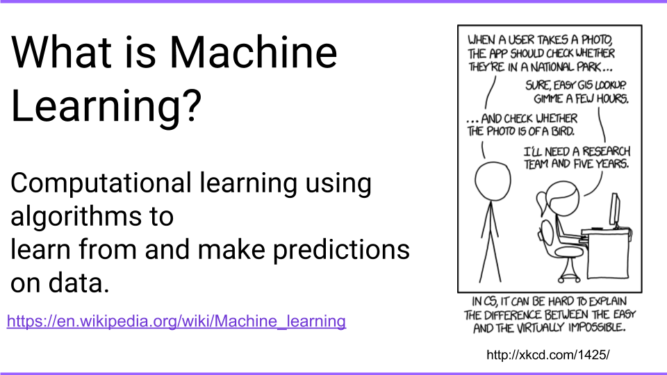 illustration from "Introduction to Machine Learning for Developers"
( blog.algorithmia.com/introduction-machine-learning-developers )
illustration from "Introduction to Machine Learning for Developers"
( blog.algorithmia.com/introduction-machine-learning-developers )
 internet meme 2017
"If managers aren't ramping up experiments in the area of machine learning, they
aren't doing their job."
— Harvard Biz Review tweet; 18 July 2017
( t.co/HwFJvlPqZT )
"LIFE IS LIKE MACHINE LEARNING — YOU NEVER KNOW WHAT YOU'RE GOING TO GET"
— an internet meme, 2017
Machine Learning (ML) seems to be the "flavor of the month." I've been jobhunting
recently and I am amazed by the number of job openings involving ML, Artificial Intelligence
(AI), Data Science and related tech. Meanwhile in the tech press there is near hysteria
about the need for companies to catch up in this new revolution.
Earlier this year I did programming work for
SQLstream, which included
integration of their streaming platform, SQLstream Blaze, with a Machine Learning
package from Apache Spark called
SystemML. They ran together on a Linux
server. Since then I got SystemML working on my MacBook Pro laptop, and have been
experimenting with it. This is a report on those experiments.
BACKGROUND
 illustration from mathworks.com
( www.mathworks.com/content/mathworks/www/en/discovery/
machine-learning/jcr:content/mainParsys/band_copy_262306852/
mainParsys/columns/1/image_2128876021.adapt.full.high.svg/1506453854867.svg )
illustration from mathworks.com
( www.mathworks.com/content/mathworks/www/en/discovery/
machine-learning/jcr:content/mainParsys/band_copy_262306852/
mainParsys/columns/1/image_2128876021.adapt.full.high.svg/1506453854867.svg )
"The [NIPS2003 Feature Selection] challenge attracted 75 competitors.
Researchers all over the world competed for 12 weeks on 5 sizable datasets
from a variety of applications, with number of input features ranking from 500
to 100,000. The goal was to use as few input features as possible without
sacrificing prediction performance. The competitors succeeded in reducing
the input space dimensionality by orders of magnitude while retaining or
improving performance. Some of the most efficient methods are among the simplest and
fastest. The benefits of using such techniques include performance improvements in
terms of prediction speed and accuracy as well as gaining better data understanding
by identifying the inputs that are most predictive of a given outcome."
— Isabelle Guyon, Steve Gunn, Asa Ben Hur, Gideon Dror
"Design and Analysis of the NIPS2003 Challenge" in
Feature Extraction, Foundations and Applications (2016)
Isabelle Guyon, Steve Gunn, Masoud Nikravesh, and Lofti Zadeh, Editors.
Series Studies in Fuzziness and Soft Computing, Physica-Verlag, Springer
( www.amazon.com/exec/obidos/ASIN/3540354875/hip-20 )
In 2001 I was invited to produce an instructional video explaining the mathematical
concept known as a Support Vector Machine (SVM), which I had previously never heard of.
The term is confusing; the "machine" refers to an algorithm, implemented in software.
What it does is called searching for "support vectors" which I will explain shortly.
The sponsor was Mindtel LLC of Rancho Santa Fe, and the knowledge came from Biowulf Corp.
I was fortunate to able to travel to Berkeley, CA and meet Isabelle Guyon, one of the
creators of the algorithm. After interviewing her and some associates, and reading a stack
of papers by her and colleagues, I came up with some metaphors for what a SVM does, and
produced a video explaining it.
If you're curious you can see the whole draft screenplay on the Mindtel web site,
(
mindtel.com/2007/0603.anakin1/HIP_images/Biowulf/biowulf_screenplay_2nd.html )
and I've been searching crates in storage lockers for the video, which I plan to
post on YouTube.
Here's one metaphor:
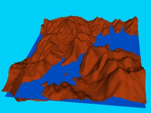 image from video "Biowulf's Mathematical Tools:
New Breakthroughs In Machine Learning" (2001)
by Alan B. Scrivener
image from video "Biowulf's Mathematical Tools:
New Breakthroughs In Machine Learning" (2001)
by Alan B. Scrivener
Imagine there's a region of terrain partially submerged by water. Let's say the water
level is at 0 feet above sea level. Let's say you have an arbitrary list of locations
in the region, with latitude and longitude (in degrees) and altitude (in feet). It might
look something like this:
| lat | lon | alt |
| 32.5 | -117.0 | 90 |
| 32.5 | -117.1 | 219 |
| 32.5 | -117.2 | -131 |
| 32.5 | -117.3 | -327 |
| 32.5 | -117.4 | -2721 |
| 32.5 | -117.5 | -3964 |
| 32.6 | -117.0 | 126 |
| 32.6 | -117.1 | 8 |
| 32.6 | -117.2 | -90 |
| 32.6 | -117.3 | -282 |
| 32.6 | -117.4 | -442 |
| 32.6 | -117.5 | -3971 |
The above data represents the bottom two rows of "pins" in this map, listed right-to-left
and bottom-to-top:
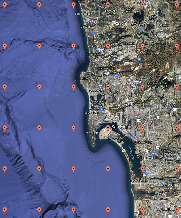 map created using https://www.darrinward.com/lat-long
If your question is, "Where is it dry or wet?" you can just look at the altitude
column and see: positive altitudes are on dry land while negative altitudes are
underwater. We can simplify the table by substituting a code: 1=wet, 2=dry, like so:
| lat | lon | wet/
dry |
| 32.5 | -117.0 | 2 |
| 32.5 | -117.1 | 2 |
| 32.5 | -117.2 | 1 |
| 32.5 | -117.3 | 1 |
| 32.5 | -117.4 | 1 |
| 32.5 | -117.5 | 1 |
| 32.6 | -117.0 | 2 |
| 32.6 | -117.1 | 2 |
| 32.6 | -117.2 | 1 |
| 32.6 | -117.3 | 1 |
| 32.6 | -117.4 | 1 |
| 32.6 | -117.5 | 1 |
If we throw in some useless columns, such as the time of day of the last measurement,
the per cent of granite in the underlying rock, or even random numbers, we're ready to
give a challenge to a Support Vector Machine.
| lat | lon | time | %
granite | random | wet/
dry |
| 32.5 | -117.0 | 28040 | 5 | 0.947522450592 | 2 |
| 32.5 | -117.1 | 46843 | 89 | 0.617269553296 | 2 |
| 32.5 | -117.2 | 4772 | 43 | 0.203837149867 | 1 |
| 32.5 | -117.3 | 4712 | 50 | 0.720961040106 | 1 |
| 32.5 | -117.4 | 68497 | 6 | 0.755910110406 | 1 |
| 32.5 | -117.5 | 60455 | 24 | 0.925103737398 | 1 |
| 32.6 | -117.0 | 25560 | 23 | 0.263836121132 | 2 |
| 32.6 | -117.1 | 39292 | 24 | 0.0865100394398 | 2 |
| 32.6 | -117.2 | 8122 | 13 | 0.170456551953 | 1 |
| 32.6 | -117.3 | 9486 | 80 | 0.849119181071 | 1 |
| 32.6 | -117.4 | 34864 | 98 | 0.990071151817 | 1 |
| 32.6 | -117.5 | 55406 | 8 | 0.730835110699 | 1 |
By way of example I'm going to talk about a Linear Binary-Class Support Vector Machine.
Linear because it only looks for linear relationships; Binary-Class because the last
column only has two possible states.
We break the dataset into two pieces (two sets of rows):
training data and
testing data.
In the case of the training data we give this data to the SVM, including the last
column, so it knows the right answers for this data. Then the magic happens, and
through advanced math, or "artificial intelligence" if you will, the SVM comes up
with a linear equation to predict the last column based on the other columns. The
testing data is used to "score" this formula for predictive value: how often is it right?
What the algorithm is going to do is to search for the "support vectors" which is to
say the important columns in the data for computing the last column. In this case one
would hope it concludes that only lat and lon are support vectors. Then it comes up
with a linear equation of the form:
score = (a * lat) + (b * lon)
where a and b are the coefficients of the support vectors. When score is negative we
have wet (1) and where it is positive we have dry (2). Since this is a linear equation it
describes a line. Looking at our map above we'd like an equation that separates the wet
from the dry cleanly, although this is not quite possible. A linear approximation is the
best the SVM can do for us.
Now, if this only worked for 2D data it wouldn't be that amazing. But you can input
much higher dimensions of data. A 3d dataset will be divided by the linear equation
of a plane. Beyond 3D it becomes very difficult to visualize, but the math is simple:
for example an 8D dataset will yield coefficients for this equation:
score = (a * x0) + (b * x1) + (c * x2) + (d * x3) + (e * x4) + (f * x5) + (g * x6) + (h * x7)
which is the equation for an eight-dimensional hyperplane dividing a hypercube. It's
a mouthful to say, but using it is easier.
You might wonder, how does it work? Honestly I have no idea. I have concentrated all
these years on how to apply it.
APACHE SystemML
 illustration for "Apache SystemML" from spark.tc
This last year I have been working with SystemML from the Apache foundation. Wikipedia
(
en.wikipedia.org/wiki/Apache_SystemML ) says:
SystemML was created in 2010 by researchers at the IBM Almaden Research Center led by
IBM Fellow Shivakumar Vaithyanathan. It was observed that data scientists would write
machine learning algorithms in languages such as R and Python for small data. When it
came time to scale to big data, a systems programmer would be needed to scale the
algorithm in a language such as Scala. This process typically involved days or weeks
per iteration, and errors would occur translating the algorithms to operate on big data.
SystemML seeks to simplify this process. A primary goal of SystemML is to automatically
scale an algorithm written in an R-like or Python-like language to operate on big data,
generating the same answer without the error-prone, multi-iterative translation approach.
On June 15, 2015, at the Spark Summit in San Francisco, Beth Smith, General Manager of IBM
Analytics, announced that IBM was open-sourcing SystemML as part of IBM's major commitment
to Apache Spark and Spark-related projects. SystemML became publicly available on GitHub
on August 27, 2015 and became an Apache Incubator project on November 2, 2015. On May 17,
2017, the Apache Software Foundation Board approved the graduation of Apache SystemML
as an Apache Top Level Project.
Algorithms in SystemML are implemented in a language called Data Manipulation Language (DML),
which looks like this:
| Xw = matrix(0, rows=nrow(X), cols=1)
debug_str = "# Iter, Obj"
iter = 0
while(continue == 1 & iter < maxiterations) {
# minimizing primal obj along direction s
step_sz = 0
Xd = X %*% s
wd = lambda * sum(w * s)
dd = lambda * sum(s * s)
continue1 = 1
while(continue1 == 1){
tmp_Xw = Xw + step_sz*Xd
out = 1 - Y * (tmp_Xw)
sv = (out > 0)
out = out * sv
g = wd + step_sz*dd - sum(out * Y * Xd)
h = dd + sum(Xd * sv * Xd)
step_sz = step_sz - g/h
if (g*g/h < 0.0000000001){
continue1 = 0 |
But you don't have to learn DML to use SystemML -- only to make changes to the algorithms.
I like SystemML because I know how to use it, it's not too hard to install and use, no
coding is required, and it runs on Linux, PC and Mac. The fact that it scales to Hadoop
clusters and Spark streams is just gravy.
All of the experiments below use Apache SystemML in Standalone mode, using the
"Binary-Class Support Vector Machines" algorithms described in section 2.2.1 of the
SystemML Algorithms Reference documentation.
(
systemml.apache.org/docs/0.12.0/algorithms-classification.html )
SystemML INSTALLATION
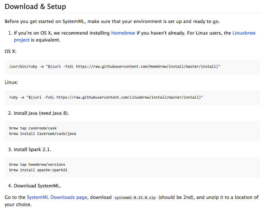 screen shot from Standalone SystemML installation instructions
( github.com/apache/systemml )
screen shot from Standalone SystemML installation instructions
( github.com/apache/systemml )
"None shall pass!"
-- the Black Knight, "Monty Python and the Holy Grail"
You too can install this free open-source software and play with it. It is easiest
on Linux, then on Mac, lastly on Windows since you must first install a bash shell
system, such as from Cygwin. I've used Linux, and most recently Mac. If you get the
software working you can follow along reproducing what I did in the sections below.
Note: Installing open-source software can sometimes seem as difficult as a Grail Quest.
Take heart that others have passed this way and survived. If you complete the quest you
will join the ranks of a few triumphant heroes. Keep calm and carry on!
To do my Mac installation I used instructions from these sources:
- I began with the instructions at Github: github.com/apache/systemml
- When, in step 3, I encountered Error: No available formula for apache-spark21
I found help here: github.com/Homebrew/homebrew-core/issues/6970
- This in turn required that I resolve brew issues, which I did with help from here: github.com/Homebrew/brew/blob/master/docs/Troubleshooting.md#troubleshooting
- I also go help from here: medium.freecodecamp.org/installing-scala-and-apache-spark-on-mac-os-837ae57d283f
- Once the installation was complete I began following the standalone tutorial on this page: systemml.apache.org/docs/0.12.0/standalone-guide
- I needed help with wget here: stackoverflow.com/questions/4572153/os-x-equivalent-of-linuxs-wget
The most important advice is be persistent, Google symptoms, and ask for help.
TEST 1: DATA FROM APACHE
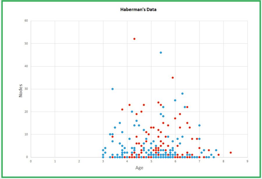 graph of Haberman data from blog post by James D. McCaffrey
( jamesmccaffrey.wordpress.com/2017/08/25/habermans-survival-data )
graph of Haberman data from blog post by James D. McCaffrey
( jamesmccaffrey.wordpress.com/2017/08/25/habermans-survival-data )
The above-linked standalone tutorial includes instructions on how to download and use test
data called the Haberman dataset, which provides four columns of data about surgery patients
for a specific procedure:
- age of a patient in years
- the xx part of the 19xx year when an operation was performed
- number of "nodes" (medical thing) detected in the patient
- the thing to predict where 1 = the patient survived for five years or more, and 2 = the patient died within five years
Here is a sample of the data:
| name: |
age |
year |
nodes |
predict |
| data row 1: | 30 | 64 | 1 | 1 |
| data row 2: | 30 | 62 | 3 | 1 |
| data row 3: | 30 | 65 | 0 | 1 |
| data row 4: | 31 | 59 | 2 | 1 |
| data row 5: | 31 | 65 | 4 | 1 |
I had installed SystemML in
~/swdev/ML/systemml-0.15.0-bin and I set the shell
variable
$SYSTEMML_HOME to point to it. In
~/swdev/ML/ I created shell
scripts as directed by the tutorial, and also created folder data_haberman containing
the data file
haberman.data.
Here is what my shell scripts do (written for the C shell
csh):
| #
printf "0.5\n0.5" > data_haberman/perc.csv
echo '{"rows": 2, "cols": 1, "format": "csv"}' > data_haberman/perc.csv.mtd
#
echo '{"rows": 306, "cols": 4, "format": "csv"}' > data_haberman/haberman.data.mtd
#
echo '1,1,1,2' > data_haberman/types.csv
echo '{"rows": 1, "cols": 4, "format": "csv"}' > data_haberman/types.csv.mtd
#
$SYSTEMML_HOME/runStandaloneSystemML.sh $SYSTEMML_HOME/scripts/algorithms/Univar-Stats.dml \
-nvargs \
X=data_haberman/haberman.data \
TYPES=data_haberman/types.csv \
STATS=data_haberman/univarOut.mtx \
CONSOLE_OUTPUT=TRUE
#
$SYSTEMML_HOME/runStandaloneSystemML.sh $SYSTEMML_HOME/scripts/utils/sample.dml \
-nvargs \
X=data_haberman/haberman.data \
sv=data_haberman/perc.csv \
O=data_haberman/haberman.part \
ofmt="csv"
#
$SYSTEMML_HOME/runStandaloneSystemML.sh $SYSTEMML_HOME/scripts/utils/splitXY.dml \
-nvargs \
X=data_haberman/haberman.part/1 \
y=4 \
OX=data_haberman/haberman.train.data.csv \
OY=data_haberman/haberman.train.labels.csv ofmt="csv"
#
$SYSTEMML_HOME/runStandaloneSystemML.sh $SYSTEMML_HOME/scripts/utils/splitXY.dml \
-nvargs \
X=data_haberman/haberman.part/2 \
y=4 \
OX=data_haberman/haberman.test.data.csv \
OY=data_haberman/haberman.test.labels.csv \
ofmt="csv"
#
$SYSTEMML_HOME/runStandaloneSystemML.sh $SYSTEMML_HOME/scripts/algorithms/l2-svm.dml \
-nvargs X=data_haberman/haberman.train.data.csv \
Y=data_haberman/haberman.train.labels.csv \
model=data_haberman/l2-svm-model.csv fmt="csv" \
Log=data_haberman/l2-svm-log_h.csv
#
$SYSTEMML_HOME/runStandaloneSystemML.sh $SYSTEMML_HOME/scripts/algorithms/l2-svm-predict.dml \
-nvargs \
X=data_haberman/haberman.test.data.csv \
Y=data_haberman/haberman.test.labels.csv \
model=data_haberman/l2-svm-model.csv fmt="csv" \
confusion=data_haberman/l2-svm-confusion.csv \
CONSOLE_OUTPUT=TRUE \
scores=data_haberman/haberman_scores |
In the script I've highlighted in red the parameters I change for each new dataset.
The number of rows is 306 and the number of columns is 4; all other red text refers to
the data directory (which I suppose I should have made a shell variable as well).
The first few rows create files in the
data_haberman directory that will be used
for the computations. The metadata (mtd) files describe the format of their sister files.
After that I invoke the provided script
runStandaloneSystemML.sh in each case,
with the algorithm provided in the DML file, such as
$SYSTEMML_HOME/scripts/algorithms/l2-svm-predict.dml.
Arguments are provided after the
-nvargs flag.
The
sampleXY and
splitXY steps create the training and testing data. The
l2-svm step trains the
SVM, and the
l2-svm-predict step tests the SVM.
Unfortunately the output from this contains a lot of error messages because I don't have
logging turned on properly, but I used a script to filter them out (available on request)
and in the resulting output I see:
Accuracy (%): 72.66666666666667
The tools also create a bunch of files in the
data_haberman directory, including:
l2-svm-model.csv
which contains the coefficients selected by the SVM:
coefficient
for age |
coefficient
for year |
coefficient
for nodes |
| 0.0011374698837280472 | -0.01232727712872697 | 0.06045232444006443 |
This makes some sense: a positive coefficient for age means a higher age results in a
greater chance of death in 5 years, as does a higher node count. A higher year (recent
surgery) results in a lower chance of death. (Remember that a negative prediction
translates to 1=lives while a positive predicition means 2=dies.)
Another file is the "confusion matrix" documented at the Apache web site
(
systemml.apache.org/docs/0.12.0/algorithms-classification.html )
but apparently they have it backwards, based my own experiments.
The generated file l2-svm-confusion.csv should contain the following confusion matrix of this form:
| Prediction ->
Actual
|
V |
1 | 2 |
| 1 | t1 | t2 |
| 2 | t3 | t4 |
The model correctly predicted label 1
t1 times
The model incorrectly predicted label 2 as opposed to label 1
t3 times
The model incorrectly predicted label 1 as opposed to label 2
t2 times
The model correctly predicted label 2
t4 times.
If the confusion matrix looks like this:
| Prediction ->
Actual
|
V |
1 | 2 |
| 1 | 107 | 38 |
| 2 | 0 | 2 |
then the accuracy of the model is (t1+t4)/(t1+t2+t3+t4) = (107+2)/(107+38+0+2) = 0.741496599
So the SVM told me its confusion matrix for the Haberman data was:
| Prediction ->
Actual
|
V |
1 | 2 |
| 1 | 100 | 8 |
| 2 | 33 | 9 |
This is how the accuracy level of 72.66666666666667 per cent above. I thought this was
pretty good until I ran across this blog entry by James McCaffrey:
(
jamesmccaffrey.wordpress.com/2017/08/25/habermans-survival-data )
Importantly, the number of survivors in the dataset is 225 and the number of people who
died is 81. So, if you just guessed "survived" (1) for every patient, you'd be correct
with 225 / 306 = 0.7353 = 73.53% accuracy.
So the SVM didn't even beat monkeys without darts!
He goes on to say:
...even a deep neural network can't really do very well on Haberman's data. The best results
I've ever gotten on Haberman's survival data use a primitive form of classification called
k-NN (k nearest neighbors). Unfortunately, some prediction problems just aren't tractable.
I wonder why such an intractable dataset was used as a beginner's first tutorial?
TEST 2: RANDOM DATA WITH A PATTERN
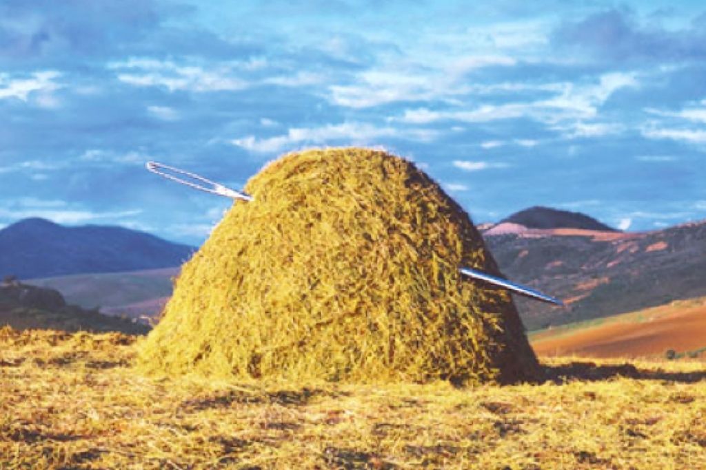 a needle in a haystack
Next I wanted to see this gizmo find a pattern I'd hidden for it.
I created a dataset, which I called
random.data, and a directory called
data_random to put it in. The dataset came from this Python program:
|
# mkMLdata.py
#
import random
#
# init vars
#
len_file = 1000
#
a1 = -0.1
a2 = 0.2
a3 = -0.3
a4 = 0.4
a5 = -0.5
a6 = 0.6
a7 = -0.7
a8 = 0.8
a9 = -0.9
#
# loop
#
for col in range (0, len_file):
#
x1=random.random()
x2=random.random()
x3=random.random()
x4=random.random()
x5=random.random()
x6=random.random()
x7=random.random()
x8=random.random()
x9=random.random()
score = a1*x1 + a2*x2 + a3*x3 + a4*x4 + a5*x5 + a6*x6 + a7*x7 + a8*x8 + a9*x9
if (score > 0.0):
sign = 2;
else:
sign = 1;
print '{0},{1},{2},{3},{4},{5},{6},{7},{8},{9}'.format(x1,x2,x3,x4,x5,x6,x7,x8,x9,sign)
|
This creates 1000 rows of 10 columns: the first nine are (pseudo) random numbers between
0.0 and 1.0, and the last uses a linear combination of the form:
score = (a * x0) + (b * x1) + (c * x2) + (d * x3) + (e * x4) + (f * x5) + (g * x6) + (h * x7) + (i * x8)
where:
a = -0.1
b = 0.2
c = -0.3
d = 0.4
e = -0.5
f = 0.6
g = -0.7
h = 0.8
i = -0.9
If score is negative then the
predict value is 1; if score is positive it's 2.
So if this SVM is any good it should be able to find these coefficients (or something like
them).
Below are some useful numbers about this dataset.
| name: |
col1 |
col2 |
col3 |
col4 |
col5 |
col6 |
col7 |
col8 |
col9 |
predict |
| my coefficient: |
-0.1 |
0.2 |
-0.3 |
0.4 |
-0.5 |
0.6 |
-0.7 |
0.8 |
-0.9 |
| svm coefficient: |
-0.434145... |
0.606559... |
-0.962973... |
1.287862... |
-1.602148... |
1.975224... |
-2.259865... |
2.786665... |
-3.161251... |
| ratios: |
4.34 |
3.03 |
3.20 |
3.21 |
3.20 |
3.29 |
3.22 |
3.48 |
3.51 |
| data row 1: |
0.184502491353 | 0.621131573599 | 0.656836128894 | 0.461035307316 | 0.58579851741 | 0.598615021871 | 0.441159402261 | 0.155037865723 | 0.355242266506 | 1 |
| data row 2: |
0.221557328333 | 0.798967758449 | 0.869295774808 | 0.585811618549 | 0.498760107223 | 0.00287997320329 | 0.459763274194 | 0.166389991898 | 0.945106431953 | 1 |
| data row 3: |
0.301930685458 | 0.859523194582 | 0.0752209472553 | 0.190349633799 | 0.66281616692 | 0.296183806467 | 0.478688042456 | 0.310067875918 | 0.418075135011 | 1 |
| data row 4: |
0.0824805682028 | 0.938126238071 | 0.64250511666 | 0.389808569647 | 0.580621341305 | 0.604629084062 | 0.282610072446 | 0.700967029877 | 0.464468514178 | 2 |
| data row 5: |
0.0569194723308 | 0.966407414661 | 0.458589233925 | 0.922457014455 | 0.207030108769 | 0.920899249796 | 0.649639261478 | 0.818377012685 | 0.177906638916 | 2 |
After I ran the SVM I was told its accuracy (in %) is 96.98795180722891, which is the
best score I've seen in this whole exercise.
The confusion matrix is:
| Prediction ->
Actual
|
V |
1 | 2 |
| 1 | 344 | 3 |
| 2 | 12 | 139 |
If you compare the "my coefficient" row with the "SVM coefficient" row, you'll see the
SVM's guesses for my coefficients. For each I calculated the ratio as well. It seems
to converge on a number near 3.5 or so.
Actually, a perfect SVM would not guess my exact coefficient, but the ratios would
all be the same. This is because the boundary of classification is defined when
score = 0, so that the formula becomes:
0 = (a * x0) + (b * x1) + (c * x2) + ...
You can multiply both sides by any constant k and the left side side is still zero, while
the right side becomes:
(k * a * x0) + (k * b * x1) + (k * c * x2) + ...
So we have to verify that the machine's coefficients are correct even after a k is multiplied.
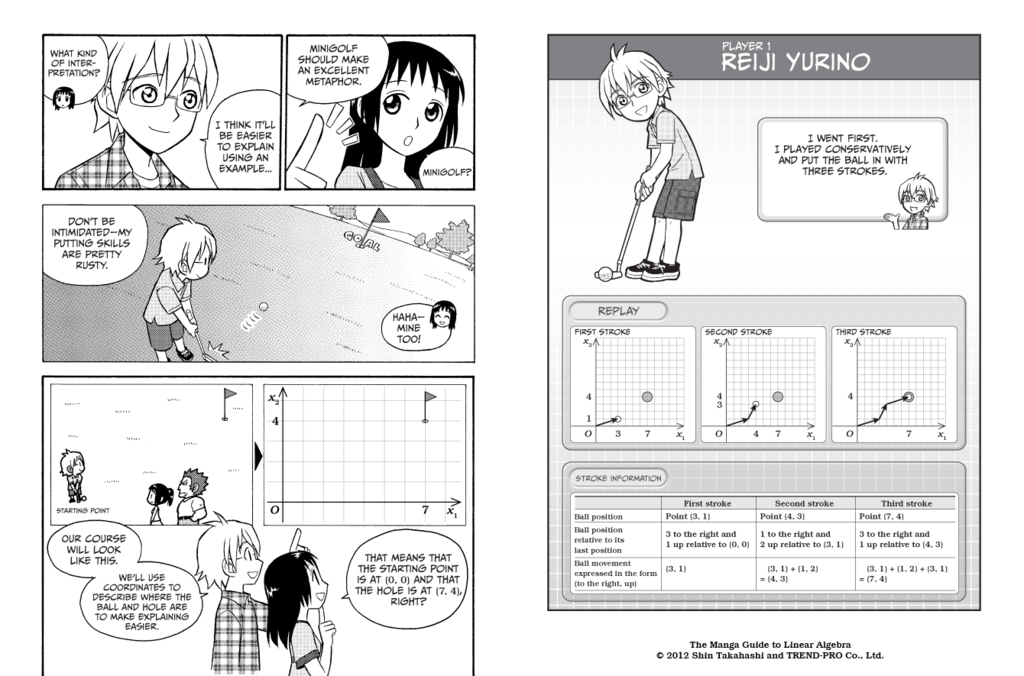
Aside: These are some of the near-magical properties of
linear equations.
To learn more I recommend the amazing math comic book "The Manga Guide to Linear Algebra"
(2012) by Shin Takahashi.
(
www.amazon.com/exec/obidos/ASIN/1593274130/hip-20 )
I noticed that the greatest deviation in the ratios was for the first column. I thought
about it and realized that if there's going to be an error somewhere, the best place to
put it is on the term that has the smallest contribution to the result, in this case
a magnitude of 0.1 out of a range of magnitudes up to 0.9. And it works OK; the
96.98... % accuracy was achieved using this coefficient with an error in it.
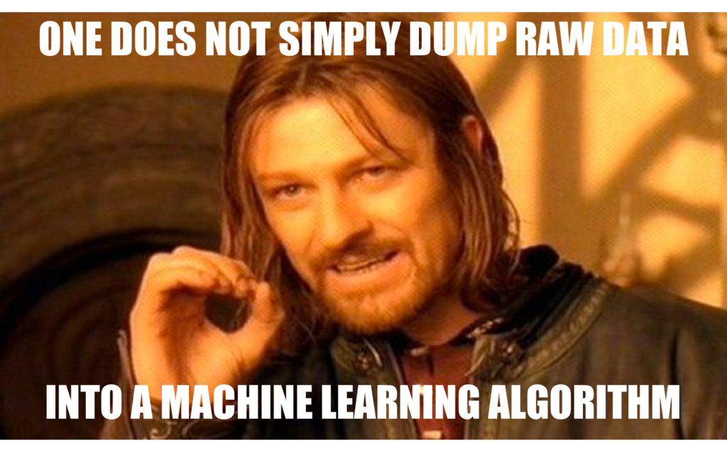
TEST 3: RANDOM DATA WITH NO PATTERN
 internet meme 2017
TYRELL: Is this to be an empathy test? Capillary dilation of the so-called
'blush response', fluctuation of the pupil, involuntary dilation of the iris.
DECKARD: We call it Voight-Kampff for short.
TYRELL: Demonstrate it. I want to see it work.
DECKARD: Where's the subject?
TYRELL: I want to see it work on a person. I want to see it work on a negative
before I provide you with the positive.
DECKARD: What's that gonna prove?
TYRELL: Indulge me.
— "Blade Runner" (movie, 1984)
Having seen it succeed, I now wanted to see the SVM fail. I modified my
Python program to output a 1 or a 2 in the predict column by (pseudo) random
choice instead of using my score equation. There was now no pattern to find.
I got an accuracy of 49.22779922779923 %, which is a little worse than random.
Not beating monkeys with darts, which could score 50 % accuracy over the long
haul.
Here is the confusion matrix:
| Prediction ->
Actual
|
V |
1 | 2 |
| 1 | 104 | 146 |
| 2 | 117 | 151 |
Well, that's a negative result alright. It occurred to me that you could get a
0.77220077220077 % boost by guessing the opposite of what the SVM predicted, but that's
probably an artifact of the dataset; more data might give a better (closer to 50%) result.
TEST 4: DISNEY STOCK DATA
 internet meme 2017
Now I was hankering to give the SVM some real data. Arbitrarily I chose stock data.
From the NASDAQ web site (
www.nasdaq.com/symbol/dis/historical )
I grabbed about 2 month's worth of daily data for The Walt Disney Company (DIS) stock.
Here are the columns I harvested:
- Date — Trading date in UNIX in epoch form (seconds since 1-1-1970) divided by 2,000,000,000
- Open — Opening price divided by 150
- High — Daily high divided by 150
- Low — Daily high divided by 150
- Close — Closing price divided by 150
- Volume — Trading volume divided by 20,000,000
- Predict — Did stock go up in the next trading day? (1=no/2=yes)
The table below shows some details of the data.
| name: |
Date |
Open |
High |
Low |
Close |
Volume |
predict |
| svm coefficient | 0.021564786755327192 | -0.14062211146101772 | -0.11012191722666322 | -0.10158773850879664 | -0.08579435131540565 | 0.46581889550920497 |
| data row 1: | 0.755136 | 0.699933333 | 0.708266667 | 0.693866667 | 0.698533333 | 0.8348745 | 1 |
| data row 2: | 0.7550928 | 0.6722 | 0.692733333 | 0.672 | 0.684533333 | 0.6529615 | 2 |
| data row 3: | 0.7550496 | 0.6792 | 0.68 | 0.669466667 | 0.674533333 | 0.4011034 | 1 |
| data row 4: | 0.7550064 | 0.675266667 | 0.686 | 0.6716 | 0.6774 | 0.6078205 | 1 |
| data row 5: | 0.7549632 | 0.6558 | 0.6742 | 0.655666667 | 0.670933333 | 0.736199 | 1 |
I ran the SVM and saw an accuracy of 38.888888888888886 %, which is
way below the
monkeys with darts. Now, I was expecting poor results from this experiment. If you
believe in the concept of "efficient markets," any information about future price that
could be this easily gleaned from available data would've already been gleaned, and the
results factored into today's price, so it wouldn't have to change tomorrow.
This logic sometimes hurts my head, reminding me of Alice in Wonderland (in the 1951
animated Disney version) who said:
If I had a world of my own, everything would be nonsense. Nothing would be what it is,
because everything would be what it isn't. And contrary wise, what is, it wouldn't be.
And what it wouldn't be, it would. You see?
But then I looked at the confusion matrix and things got, as they say, curiouser and
curiouser:
| Prediction ->
Actual
|
V |
1 | 2 |
| 1 | 12 | 2 |
| 2 | 17 | 1 |
In almost every case the SVM predicted the stock would not go up. Since the stock did
go up more often than not (18 out of 32 times) in the testing data, this was disastrous
for the SVM. Now, in the training data the stock went up only 15 out of 33 times, so
what we are seeing is a shift in the pattern (if there really is a pattern) happening
fast enough to confound the SVM.
NEXT STEPS
 illustration from SAP Analytics Twitter feed
( twitter.com/SAPAnalytics/status/788204197116280832 )
illustration from SAP Analytics Twitter feed
( twitter.com/SAPAnalytics/status/788204197116280832 )
I wanted to put these results out there, so that others may use them, but there are things
I still want to do:
- better data
I feel like I haven't had a real "win" yet with this technique. From my years in
visualization I've learned that people love a good story, coupled with the right
balance of surprise and confirmation. There's a sweet spot between obvious and
incomprehensible. Most people know the story of beer next to the diapers;
( canworksmart.com/diapers-beer-retail-predictive-analytics )
though the real story is less dramatic, but this is an example of the kind of stories
we want to be told about machine learning, despite the fact that the machines really
can't provide them. As quoted above, "LIFE IS LIKE MACHINE LEARNING — YOU NEVER
KNOW WHAT YOU'RE GOING TO GET." One of the added values of data analysts in this era
seems to be pulling together good stories.
- simulate purchase data
A tricky problem with classifiers is getting good data into the prediction column in
a timely way. The example everyone seems to want to explore these days is credit
card fraud, but the [problem is that when someone sticks a card into a slot —
and you have maybe 5 seconds to decide whether to decline it — all of the
data on the integrity of that transaction is not yet available. Fraud often gets
caught days later when someone checks their bill. To do a useful job, this data must
be folded into the training and testing data, so that the SVM "knows the future"
while it is learning. The analyst groups such as Forrester are getting all excited lately
about real-time systems being retrained on the fly, but this can't work if accurate data
cannot be provided in real-time for the prediction column.
One idea I've had is to use sales data from vending machines with variable pricing.
The predicted event is a sale, and that data is available immediately. Ideally I'd
love to get my hands on real, raw data, but the vending machines are still mostly
stuck in a mode where it takes a service visit to change pricing. Look for more variable
pricing data as new machines roll out. But meanwhile, simulating purchases may be useful.
A swarm of "sims" wandering a stylized shopping center past vending machines, each with
a shopping list and a price-sensitivity function ("demand curve"), could provide training
and testing data for experiments while waiting on real data.
- experiment with higher-order nonlinear terms
Though the solver I'm using is linear, Isabelle Guyon once clued me in that you can make
them non-linear by adding columns combining other columns. For example, assuming that
people enjoy hot chocolate more with marshmallows more than they enjoy either with
pickles, we would expect that if besides chocolate (c), marshmallows (m) and pickles (p)
columns we add the products cm, cp and mp, we would expect the cm column to have more
weight. (For such products of columns it is advisable to scale them from 0.0 to 1.0
first.)
Also, a square function has a "U" shape (or, if negated, a "hump" shape) which makes
finding correlations with hump-shaped patterns easier.
- investigate Kaggle
I learned at a recent San Diego Python meetup that there is a project called "kaggle"
which has data analytics contest on-line, and "leader boards" of the best analysts for
each contest. I'm going to look into this, for the data sources, the experience, and
possibly the glory.
( www.kaggle.com )
Note Re:
"If It's Just a Virtual Actor,
Then Why Am I Feeling Real Emotions?"
Part eight of this serialization will appear next time.
TO BE CONTINUED...
========================================================================
newsletter archives:
www.well.com/user/abs/Cyb/archive
========================================================================
Privacy Promise: Your email address will never be sold or given to
others. You will receive only the e-Zine C3M from me, Alan Scrivener,
at most once per month. It may contain commercial offers from me.
To cancel the e-Zine send the subject line "unsubscribe" to me.
~~~~~~~~~~~~~~~~~~~~~~~~~~~~~~~~~~~~~~~~~~~~~~~~~~~~~~~~~~~~~~~~~~~~~~~~
I receive a commission on everything you purchase from Amazon.com after
following one of my links, which helps to support my research.
========================================================================
Copyright 2017 by Alan B. Scrivener
Last update:
Wed Dec 20 11:40:00 PST 2017