
Last update: 15-Jun-1997
Even before there were computer graphics, I enjoyed playing with mathematical puzzles and games. The first vector was drawn by computer in the early sixties; shortly before the hidden line problem was solved in the early seventies, I began playing with using computers to illuminate mathematics. I've never been able to stop.
I created the letters of this polygonal alphabet in 1984 to use to test rendering hardware, and I've been carrying them around ever since.

These are algorithmically simple, yet very beautiful in my opinion.
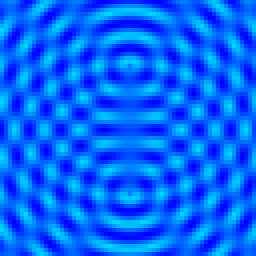
Moire patterns fascinate me, and I simulate them on every graphics system I program. What once took a weekend to compute on an Apple II can now go at real-time frame rates on an SGI Indogo 2.
v = sin(sqrt(xc1 - x)^2 + (yc1 - y)^2)
  + sin(sqrt(xc2 - x)^2 + (yc2 - y)^2)
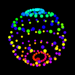
This was a lunch-hour hack in 1988, inspired by an article in Scientific American.
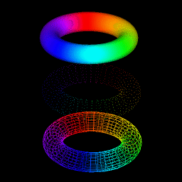
x = R*sin(A*t)*cos(B*t)
y = R*sin(A*t)*sin(B*t)
z = R*cos(A*t)
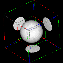
This is an illustration for a paper I have submitted for SIGGRAPH '96 in New Orleans. (See http://siggraph.org/ for more information on the conference.) The picture is a 4-D visualization of a light cone (from Einstein's Special Relativity Theory) mapped onto a tesseract (unfolded hypercube).
sqrt(x^2 + y^2 + z^2 - t^2) = K
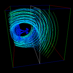
Since college I have been interested in systems theory, and how dynamical systems evolve by the "change rules" of Ordinary Differential Equations (ODEs). By mapping a 2-D or 3-D state space into a graphical representation, it is is possible to see many possible system behaviors at once, each represented by a trajectory through the space. Here are some systems I have visualized this way:
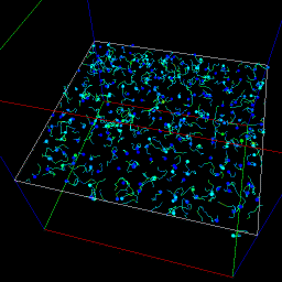
The change vector at each point in the volume is randomly assigned.
xdot = rand(x, y, z)
ydot = rand(x, y, z)
zdot = rand(x, y, z)
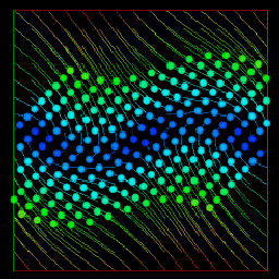
A simple 2-D system that loses energy as it oscillates, seeking one of two stable equilibrium points. (A third unstable equilibrium point sits beteen them.)
xdot = y
ydor = sin(x) - y
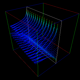
A more complex 3-D system that finds an oscillating equilibrium.
xdot = y
ydot = -(x + y^3 - y) + cos(z)
zdot = K

K = 8
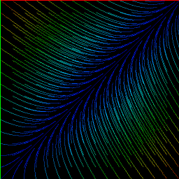
A 2-D simulation of two nations in an escalating arms race, each responding to the other's arms buildup.
xdot = -A*x + B*y + C
ydot =  D*x - E*y + F

A = B = C = D = E = F = 0.5
The famous 3-D system of thermal convection that exhibited some of the first chaos ever recognized in a mathematical model.
xdot = A*(y - x)
ydot = B*x - y - (x*z)
zdot = x*y - C*z

A = 10
B = 28
C = 5/3
Return to to ABS's home page.