Steps to running the model:

• download the software
  • A run time version of the modeling software is available free from High Performance Systems.
• download the model
  • Click here - you will be prompted to save it on your computer
• install the software
• double click on the model

Getting Started

1. When the model opens you should see a graph with three straight lines which have an oscillation in the middle which then smooth out. If you don't see a graph, press 'Control H'. Pressing 'Control R' will start the model running. Since the default mode is equilibrium the lines will stay flat. Click on the triangle at the bottom left of the graph pad to see other pages. (You can do this while the model is running).

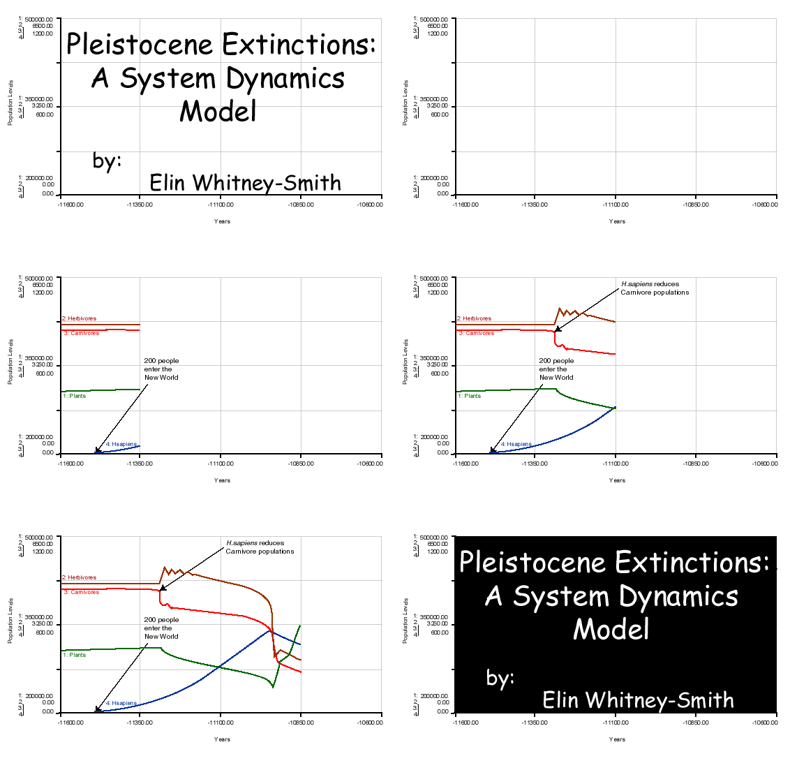
   The chart pad will appear and disappear with the graph pad. Clicking on the triangle at the bottom left of the chart will show other pages of the chart. If you cannot see the chart pad it may be covered by the graph pad. Move the graph pad by clicking and dragging on the upper edge or resize by clicking and dragging the border.

2. The first slider controls the number of people entering the New World. The default is set at 200 (0.2K) following the model done by Whittington and Dyke (1989). Click on the 'U' button to run the model in default Overkill mode. Look at what happens if 1000 people enter the new world. Look at what happens if 10,000 do.
   Click on the 'U' button to reset to the default value.

3. The second slider controls how much people reduce carnivore populations. The default value is 2% (0.02). Click on the 'U' button on the second slider. Press 'Control R' to start the model. Look at the other pages of the graph pad to see what is happening with Herbivores and Vegetation.

   Now see what happens if people reduce carnivore populations by 4% (0.04) (Note: It may be easier to place your cursor in the little window in the slider and type in the number. You have to press enter before the change will work.)

   Now see what happens when people only reduce carnivore populations by 1%(0.01). As you see there is no extinction. Running the model this way and then running the model in simple Overkill mode gives a clue to why people would be motivated to reduce carnivore populations.

   In the short term H. sapiens populations establish themselves more quickly when they reduce carnivore populations. There are more herbivores and fewer carnivores so people have more to eat. It is only in the long term, if carnivore reduction has exceeded the threshold value (1.5% or so in this model), that extinctions occur.
   Click on the 'U' button to reset to the default value.

4. The third slider controls how soon after people enter the New World they start to reduce carnivore populations. The default is 200 years. If carnivore populations are reduced earlier the extinctions take less time. If they are reduced later they take longer. The end result is the same but the path is different. The earlier the reduction takes place the greater the boom and the sooner the crash. If the reduction takes place later H. sapiens has a chance to establish a population which then crashes. To change the number of years the simulation runs, go to the 'Run' menu and select 'Time Specs'. This will bring up a box which allows you to change the run time. Use the same method to return the model run time to the original or close the model.

5. The fourth slider controls how many pounds of herbivore is necessary to support one pound of H. sapiens per year. The default - 10 lbs. - is half what it takes to support a carnivore. See what happens if you reduce the amount to 5 lbs. Now see what happens if you increase it to the same amount as a non-human carnivore - 20 lbs. - now increase it to more than a non-human carnivore - 30 lbs. Try this running the model under Overkill (H. sapiens do not reduce carnivore populations) and Second Order Overkill (H. sapiens reduce carnivore populations) modes. (Note: in this experiment it is advisable to increase the time period of the model.)

   Whittington and Dyke (1989) extrapolated how much a person would have to hunt to effect extinction. They came up with 38.6 pounds of prey per pound per year. Let us run the model at 40 lbs. twice the amount of prey needed by a non-human carnivore. The model begins to oscillate in both modes. Presumably during the periods of extreme oscillation the less efficient of each kind of animal would suffer and some would go extinct but there is no bias in favor of ruminants.

You have completed the first level of interacting with the model.

To interact with these variables:

• Click on the '?' button to see the documentation. You will notice that some of the graphs do not have a '?' button. These are variables related to grazers, ruminant and non-ruminant. I have supplied the documentation in the box surrounding the graph.

• Double click on the graph to change the slope of the curve. Most of the changes I have experimented with make the entire model unstable but do not make Overkill more likely.

• The easiest way to make the model unstable is to change the slope of the curve controlling how the environment is apportioned to trees and grass.

• The easiest way to prevent extinctions when running in Second Order Overkill mode is to match the H. sapiens hunting curves to the Carnivore hunting curves. The current configuration assumes that H. sapiens is more apt to switch to gathering when herbivores are scarce and to loose interest when they can obtain the maximum number of herbivores to support existing populations and reproduce at a maximum rate.

If you find an combination which is stable and which makes Overkill more likely than Second Order Overkill please e-mail me at elin@quaternary.net

References

1989. Simulating overkill: experiment with the Mossiman and Martin model. In, Martin, P.S. & Klein, R.G. (eds) Quaternary extinctions: A prehistoric revolution. Univ. Arizona Press, Tucson